Empirical Likelihood for Change-point Detection using Double Quantile (졸업연구논문)
석사 졸업 연구 논문
졸업 논문이 본심을 통과하면서 2년의 석사 과정을 마치게 되었습니다. 석사 졸업 연구 주제인 ‘Change-point detection using Nonparametric methods’에 대해 적어보려 합니다.
-
논문
‘Empirical Likelihood for Change-point Detection using Double Quantile’ Danah Kim, Master thesis, Graduate School, Yonsei University, 2020
→ URL -
통계학회 참여 및 수상 후기
→ 바로가기
1. Introduction
1.1. Backgrounds of Change-point Problem
변경점(Change-point)은 시간의 흐름에 따른 일련의 과정에서 통계적 특성이 근본적으로 변화하는 지점을 의미합니다. 프로세스의 통계적 속성이 변화하는 순간으로 변동점이라고도 불립니다.

제조, 금융, 역학 등 다양한 분야에서 변경점이 발생했는지, 그리고 발생했다면 그 위치가 어디인지 파악하는 문제는 중요한 연구 주제였습니다. 통계적 공정 관리(Statistical Process Control)의 창시자로 알려진 W. A. Shewhart는 1931년에 불량률 관리의 목적으로 관리도(Control Chart)를 처음 개발하였습니다. 관리도에서 UCL(Upper Control Limit)과 LCL(Lower Control Limit)은 프로세스 변동의 상한과 하한을 나타내는 중요한 기준선입니다. 만약 관측치가 UCL 또는 LCL을 초과하거나 미달하면 이는 프로세스에 통계적으로 유의미한 변화가 발생했음을 의미하며, 즉시 조치를 취해야 할 가능성이 있습니다.
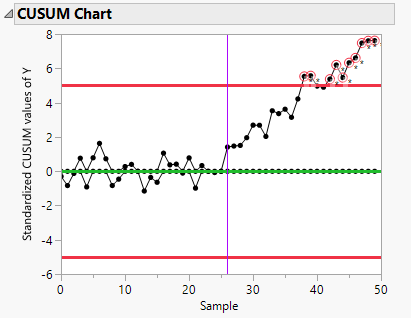
CUSUM 차트는 누적합 제어도(Cumulative Sum Control Chart)로, 1954년에 E.S. Page에 의해 개발되었습니다. 각 관측치가 누적되면서 목표값(예를들어 평균값)에서 벗어나는 정도를 추적합니다. 이것은 작은 변화가 반복되더라도 차트에서 점진적으로 누적되어 변화를 빨리 알아챌 수 있게 도와줍니다. 이러한 변경점 탐지 방법들은 이후 많은 연구의 초석이 되었습니다.
변화를 감지하는 방법에는 크게 온라인(online)과 오프라인(offline) 방식이 있으며, 각각의 방식은 데이터가 어떻게 수집되고 분석되는지에 따라 적용 방법이 다릅니다.
온라인 변경점 탐지(Online Change-point Detection)는 실시간으로 데이터를 분석하여 즉각적으로 변화점을 감지하는 방법입니다. 스트리밍 데이터에 적합하며, 변화가 발생하면 빠르게 대응할 수 있다는 장점이 있습니다. CUSUM과 EWMA 같은 기법들이 대표적입니다.
반면, 오프라인 변경점 탐지(Offline Change-point Detection)는 모든 데이터를 수집한 후에 변화를 분석합니다. 더 정밀한 변환점 탐지가 가능하며, 다양한 통계적 또는 머신러닝 기법을 적용할 수 있습니다. 대표적으로 Dynamic Programming과 Bayesian 방법, Likelihood Ratio Test가 있으며, 변화의 패턴과 정확한 위치를 분석할 수 있다는 장점이 있습니다.
본 연구에서는 Likelihood Ratio Test를 이용하여 통계적으로 검정하는 오프라인 변경점 탐지 방법에 대해 연구합니다.
1.2. Change-point Problem
변경점 문제에 대한 정의는 다양하지만, 본 연구에서는 다음과 같이 정의합니다.
일련의 관측값 $x_{1}, x_{2}, \ldots, x_{n}$이 독립적인 확률 변수 $X_{1}, X_{2}, \ldots, X_{n}$로부터 추출된다고 가정합니다. 데이터에는 여러 개의 변경점 $\tau_{1}, \tau_{2}, \ldots , \tau_{m}$이 존재하며, 그로 인해 $(m+1)$개의 구간이 형성됩니다. 이때 일련의 관측값의 분포는 다음과 같이 표현됩니다.
\[X_{i} \sim \begin{cases} & F_{1} \; \; \; \; \text{ if $i \le \tau_{1}$} \\ & F_{2} \; \; \; \; \text{ if $\tau_{1} < i \le \tau_{2}$} \\ & \vdots \\ & F_{m+1} \; \text{ if $\tau_{m} < i$} \end{cases}\]즉, 변경점 문제는 변경점 $\tau$가 $\tau_{1}$부터 $\tau_{m}$까지 $m$개 존재할 때, $F_{1}$부터 $F_{m+1}$까지 $m+1$개의 분포로 나눠진다는 가정하에 시작합니다. 이러한 분포 구조의 변화는 주로 평균, 분산, 또는 분포 자체의 변화로 나타납니다. 따라서 변경점 문제에서 $\tau$의 위치와 개수를 정확하게 탐지하는 것이 핵심입니다.
1.3. Change-point Model
변경점 문제를 해결하기 위해 $\tau$의 적절한 위치와 개수를 탐지하기 위한 통계적 모델을 정의합니다. 먼저 $\tau$에서 단일 변화가 존재한다고 가정합니다. 이렇게 단일 변경점을 탐지한 후, 해당 지점을 기준으로 앞뒤로 이진 세분화(binary segmentation)를 반복적으로 수행하면 모든 변경점을 찾을 수 있습니다. 이를 통해 변경점 탐지 문제는 단일 변경점을 탐지하는 문제로 단순화할 수 있습니다.
독립적인 확률 변수 $X_{1} \sim G_{1}, \ldots, X_{n} \sim G_{n}$을 고려합니다. 위의 분포에서 최대 하나의 변경점 $\tau$가 존재한다고 가정합니다. 우리는 변화가 없다는 귀무 가설을 검정하고자 합니다.
\[\label{eq1}\tag{1} \mathbf{H_{0}} : G_{1} = G_{2} = \ldots = G_{n} = F,\]이에 대해 단일 변경점이 존재한다는 대립 가설은 다음과 같습니다.
\[\label{eq2}\tag{2} \mathbf{H_{a}} : F_{1} = G_{1} = G_{2} = \ldots = G_{\tau} \ne G_{\tau+1} = \ldots = G_{n} = F_{2}.\]여기서 $1 \le \tau < n$이며, $F$와 $G$는 어느 것도 퇴화하지 않는다고 가정합니다. 이진 세분화를 통해 각 단계에서 순차적으로 단일 변경점의 위치를 추정하고 검정하는 것이 적절합니다.
2. Proposed Methodology
2.1. Statistical Methods on Change-point Analysis
위에서 설명한 Model에서 변경점을 탐지하는 방법을 크게 통계적으로 모수적 방법과 비모수적 방법으로 나눌 수 있습니다. 모수적 방법 중 연구가 가장 많이된 분야는 정규분포에서 평균의 변화에 대한 탐지이며, 분산의 변화에 대해서도 연구가 되고 있습니다.
그러나 (1) 모수적 가정은 때때로 현실에서 만족되지 않습니다. 이는 실제 데이터가 가정된 분포에서 벗어나는 경우 분석 결과의 신뢰도가 크게 떨어질 수 있다는 것을 의미합니다. 또한 (2) 이상치(outlier)에 민감하며, 특히 이상치는 모형의 모수 추정에 큰 영향을 미쳐 분석의 정확성을 저해할 수 있습니다. 이는 이상치가 평균이나 분산과 같은 모수를 왜곡시켜, 결과적으로 분석의 신뢰성을 떨어뜨리기 때문입니다. 예를 들어, 평균의 변화 탐지 시 이상치가 존재하면 실제 변화와 무관하게 평균이 크게 변하게 되어 잘못된 결론을 도출할 수 있습니다. 그리고 (3) 극단에 위치한 값은 분포에 따라 크게 다르다는 한계점이 존재합니다. 이는 극단값이 데이터의 특성에 큰 영향을 미칠 수 있으며, 가정된 분포 구조가 왜곡될 수 있음을 의미합니다.
반면, 비모수적 방법은 가정이 훨씬 적고 다양한 상황에 더 적합하게 적용될 수 있습니다. 이는 데이터가 특정한 분포를 따른다고 가정하지 않기 때문에, 분포에 대한 사전 지식이 없거나 데이터의 분포가 복잡한 경우에도 유연하게 적용될 수 있다는 장점이 있습니다. 또한 비모수적 방법은 이상치나 극단값의 영향을 덜 받으며, 데이터 자체에 기반한 추론을 수행하기 때문에 현실적인 상황에서 더 강건한 결과를 제공할 수 있습니다.
비모수적 방법으로도 변경점에 대한 많은 연구가 이루어졌으며, 2007년에는 경험적 가능도 비율(Empirical Likelihood Ratio)을 이용한 변경점 문제에 대한 연구와 2017년에 제안된 분위수 경험적 가능도(Quantile Empirical Likelihood) 방법을 발전시켜, 이번 연구에서는 양 방향으로의 이중 분위 경험적 가능도(Double quantile empirical likelihood)를 제안합니다.
2.2. Empirical Likelihood
본 연구에서 사용한 비모수적 방법론은 경험적 가능도(Empirical Likelihood)입니다. Art B. Owen은 1988년에 비모수적 방법으로 경험적 가능도를 처음 제시했으며, 주요 개념은 각각의 관측치에 미지의 확률 질량(unknown probability mass)을 부여하는 것 입니다.
독립적이고 동일하게 분포된 관측값 $x_{1}, \ldots, x_{n}$이 알려지지 않은 모집단 분포 $F$에서 추출되었다고 가정합니다. 이때 $p_{i} = P(X=x_{i})$라고 정의하면, ${ p_{i} }_{i=1}^{n}$의 경험적 가능도 함수는 다음과 같습니다.
\[L(F) = \prod_{i=1}^{n} p_{i},\]여기서 $p_{i}$는 $p_{i} \ge 0$ 및 $\sum_{i=1}^{n} p_{i}=1$의 제약 조건(constraints)을 만족합니다.
따라서 $L(F)$는 $p_{i}=1/n$일 때 최대가 되며, 전체 모델(Full Model)에서 $n^{-n}$이 최대값을 갖습니다.
모집단 모수 $\theta$가 $E[m(X;\theta)]=0$으로 정의될 때, $\theta$가 참값 $ \theta_{0}$을 가질 경우 추가 제약 조건을 만족하면서 경험적 가능도를 최대화할 수 있습니다.
\[\sum_{i=1}^{n} p_{i} m(x_{i},\theta_{0}) = 0.\]이와 같은 제약식을 추가하여 각 관측치에 대한 확률을 최대화할 수 있습니다. 이러한 최적화 문제는 라그랑주 승수법(Lagrange multiplier)을 사용하여 풀 수 있습니다.
제약 조건 하에서 ${p_{i}}_{i=1}^{n}$을 찾기 위해 라그랑주 승수법을 적용하면 다음과 같은 식을 얻을 수 있습니다.
\[\sum_{i=1}^{n} \log p_{i} + \lambda_{0} ( \sum_{i=1}^{n} p_{i} - 1) + \lambda_{1} (\sum_{i=1}^{n} p_{i} m(x_{i},\theta_{0})).\]따라서 경험적 가능도 비율(ELR)은 다음과 같이 정의됩니다. 이는 근사적으로 카이제곱 분포(Chi-squared distribution)를 따른다고 알려져 있습니다. 경험적 가능도 방법은 라그랑주 승수법을 사용하여 다른 제약 조건을 추가적으로 고려할 수 있습니다.
$\theta = \theta_{0}$를 검정하기 위한 경험적 가능도 비율 통계량(Empirical Likelihood Ratio(ELR) statistic)은 다음과 같습니다. \(\mathbf{R(\theta_{0})} = \frac{L(F)}{L(F_{n})} = \max \left ( \prod_{i=1}^{n} np_{i} | \sum_{i=1}^{n} p_{i}m(x_{i}, \theta_{0})=0, p_{i} \ge 0, \sum_{i=1}^{n} p_{i} =1 \right )\)
Under the null model $\theta = \theta_{0}$ with mild regular conditions, $-2 \log \mathbf{R(\theta_{0})} \to \chi_{r}^{2}$ in distribution as $n \to \infty$, where $r$ is dimension of $m(x, \theta)$ (Owen, 1988). The empirical likelihood method can be extended to other constraints using Lagrange multiplier method to find $\{p_{i}\}_{i=1}^{n}$.
2.3. Empirical Likelihood for Two Groups Comparison
위의 검정 방법을 두 그룹 비교 검정(Two Groups Comparison Test)으로 확장할 수 있습니다. $F_{1}$과 $F_{2}$의 확률을 최대화하는 경험적 가능도(Empirical Likelihood)를 정의하면, 이표본 검정(Two-sample Test)으로 변경점을 이진적으로 두 개의 분포로 나누는 검정과 동일하게 됩니다.
두 샘플: $X_{1}, X_{2}, \ldots, X_{n} \sim F_{1}$ 그리고 $Y_{1}, Y_{2}, \ldots, Y_{m} \sim F_{2}$이며, $p_{i} = P(X=x_{i})$, $q_{j} = P(Y=y_{j})$로 정의합니다. $p_{i}$와 $q_{j}$의 경험적 가능도 함수는 다음과 같이 정의됩니다.
\[L(F) = \prod_{i=1}^{n} p_{i}\prod_{j=1}^{m} q_{j},\]where $p_{i}$ and $q_{j}$ satisfy the constraints $p_{i} \ge 0, q_{j} \ge 0$ and $\sum_{i=1}^{n} p_{i}=1$, $\sum_{j=1}^{m} q_{j}=1$.
식 (\ref{eq1}), 식 (\ref{eq2})와 동등한 검정입니다.
\[\mathbf{H_{0}} : F_{1} = F_{2},\]이에 대한 대립 가설은 다음과 같습니다.
\[\mathbf{H_{a}} : F_{1} \ne F_{2}.\]따라서 이 가설은 이표본 검정 문제(Two-sample Test)로 귀결됩니다.
2.4. Quantile Llikelihood Ratio for Two Sample
Zhou, Y., Fu, L., and Zhang, B.(2017) 논문에 따르면 분위(quantile)를 이용한 제약 조건(constraints)을 경험적 가능도(empirical likelihood)에 추가하여 확률을 추정할 수 있습니다.
귀무 가설 하에서, 주어진 $x$에 대해 $F_{1}(x) = F_{2}(x) = F(x)$가 성립합니다. $p=F(\xi_{p})$라고 할 때, $\xi_{p}$는 $F$의 $p$ 분위이며, $\xi_{p}$는 다음 조건을 만족해야 합니다.
\[\label{eq3}\tag{3} E[I(X_{i} \le \xi_{p})-p]=0, \quad \text{for } 1 \le i \le n+m\]이를 이용해 다음과 같은 제약 조건 하에서 분위 경험적 가능도 검정 통계량(quantile empirical likelihood test statistic)을 구성할 수 있습니다.
\[\mathbf{R(\xi_{p})} = \max \left ( \prod_{i=1}^{n} np_{i} \prod_{j=1}^{m} mq_{j} | \sum_{i=1}^{n} p_{i} I(X_{i} \le \xi_{p}) ) = p, \right .\] \[\left . \sum_{j=1}^{m} q_{j} I(Y_{j} \le \xi_{p}) ) = p, p_{i}, q_{j} \ge 0, \sum_{i=1}^{n} p_{i} = \sum_{j=1}^{m} q_{j} =1 \right )\]이를 확장하여 제안하는 방법이 이중 분위 가능도(Double quantile likelihood)입니다. 이는 앞서 언급한 경험적 가능도(empirical likelihood)에서 좌측과 우측의 분위(quantile)를 제약 조건(constraints)으로 사용하여 추정하는 방법입니다. 두 개의 분위을 사용하여 경험적 가능도를 최대화합니다.
식 (\ref{eq3})를 양 극단에 모두에 대해 확장한 $\textbf{Double quantile likelihood}$로 정의됩니다. $p=F(\xi_{p})$와 $1-q=F(\xi_{1-q})$라 할 때, $\xi_{p}$는 $F$의 $p$ 분위이고, $\xi_{1-q}$는 $F$의 $1-q$ 분위에 해당하는 값입니다. 이는 다음을 만족합니다. \(\label{eq4}\tag{4} E[I(X_{i} \le \xi_{p})-p]=0, \quad E[I(X_{i} \ge \xi_{1-q})-q)]=0\)
where $0 < p < 1-q < 0$ for $1 \le i \le n+m$.
식 (\ref{eq4})를 이용해 제약 조건 하에서 이중 분위 경험적 가능도 검정 통계량(double quantile empirical likelihood test statistic)은 다음과 같이 정의됩니다.
\[\label{eq5}\tag{5} \mathbf{R(\xi_{p}, \xi_{1-q})} = \max \left ( \prod_{i=1}^{n} np_{i} \prod_{j=1}^{m} mq_{j} | \sum_{i=1}^{n} p_{i} I(X_{i} \le \xi_{p}) )=p, \right .\] \[\sum_{j=1}^{m} q_{j} I(Y_{j} \le \xi_{p}) )=p, \sum_{i=1}^{m} q_{i} I(X_{i} \le \xi_{1- q}) )=1-q,\] \[\left . \sum_{j=1}^{m} q_{j} I(Y_{j} \le \xi_{1-q}) )=1-q, p_{i}, q_{j} \ge 0, \sum_{i=1}^{n} p_{i} = \sum_{j=1}^{m} q_{j} =1 \right )\]라그랑주 승수법(Lagrange multiplier)을 통해 유일한 라그랑주 승수($\lambda$)를 구하고 이를 통해 확률을 추정합니다. 따라서 유도된 이중 분위 가능도 비율(DLR)는 위와 같습니다. 이때 이 검정 통계량(test statistic)을 최대화시키는 $\xi_{p}$와 $\xi_{1-q}$를 선택하며, 큰 검정 통계량 $D_{n}$은 적어도 하나의 변경점이 존재할 가능성이 크다는 것을 의미하고, 귀무 가설의 기각을 의미합니다. 증명은 Appendix.A에 수록되어 있습니다.
라그랑주 승수법을 사용하여 식 (\ref{eq5})를 풀면, 다음과 같은 유일한 $\lambda$와 $p_{i}$, $q_{j}$를 얻을 수 있습니다(증명은 Appendix.A에 포함). 이는 이중 분위 가능도 비율(DLR) 검정 통계량으로 이어집니다.
\[\begin{gathered} \mathbf{R(\xi_{p}, \xi_{1-q})} = \left ( \frac{np}{n_{1}} \right )^{n_{1}} \left ( \frac{nq}{n_{2}} \right )^{n_{2}} \left ( \frac{n(1-p-q)}{n-n_{1}-n_{2}} \right )^{n-n_{1}-n_{2}} \\ \left ( \frac{mp}{m_{1}} \right )^{m_{1}} \left ( \frac{mq}{m_{2}} \right )^{m_{2}} \left ( \frac{m(1-p-q)}{m-m_{1}-m_{2}} \right )^{m-m_{1}-m_{2}} \end{gathered}\]where $\sum_{i=1}^{n} I(X_{i} \le \xi_{p}) = n_{1}$, $\sum_{i=1}^{n}I( X_{i} > \xi_{1-q}) = n_{2}$ and $\sum_{j=1}^{m} I(Y_{j} \le \xi_{p}) = m_{1}$, $\sum_{j=1}^{m}I( Y_{j} > \xi_{1-q}) = m_{2}$
\[\therefore D_{n} = \sup_{\xi_{p}<\xi_{1-q}} \{ -2\log \mathbf{R(\xi_{p}, \xi_{1-q})} \}\]큰 $D_{n}$ 값은 적어도 하나의 변경점이 존재함을 나타냅니다.
3. Simulations
3.1. Algorithm for Change-point Detection
본 절에서는 제안된 DLR을 이용한 변경점 탐지 알고리즘을 설명합니다. 변경점 $\tau$는 이표본 검정(two-sample test)인 DLR을 통해 추정할 수 있습니다.이때 $F_{1}$과 $F_{2}$의 샘플 크기가 너무 작을 경우, 경험적 가능도(Empirical Likelihood, EL)의 추정치인 라그랑주 승수($\lambda$)가 존재하지 않을 수 있습니다. 따라서 2007년 Zou의 논문에서 제시된 trimming 방법을 사용하여 샘플 크기 $n$과 $m$을 조정하고, 조정된 통계량 $D_{n}^{*}$을 이용해 변경점을 추정합니다. 이때 $D_{n}^{*}$를 가장 최대화하는 $\tau$를 변경점으로 추정합니다.
변경점 탐지 문제는 다음과 같은 $\tau$를 탐지하는 문제로 정의됩니다.
\[F_{1} = G_{1} = G_{2} = \ldots = G_{\tau} \ne G_{\tau+1} = \ldots = G_{n} = F_{2}\]두 샘플 검정에서는 $X_{1}, \ldots, X_{n} \sim F_{1}$ 그리고 $Y_{1}, \ldots, Y_{m} \sim F_{2}$라고 가정합니다. 만약 $n$ 또는 $m$이 너무 작다면, 경험적 가능도 추정치인 라그랑주 승수가 존재하지 않을 수 있습니다. 이러한 경우에는 trimming된 통계량(Zou, C. 2007)을 사용합니다.
\[D_{n}^{*} = \sup_{ c(n+m)^{-1/9}<\xi_{p}<\xi_{1-q}<1-c(n+m)^{-1/9} } \{ -2\log \mathbf{R(\xi_{p}, \xi_{1-q})} \}\]where $c$ is a positive constant.
변경점 $\tau$ 는 다음과 같이 추정할 수 있습니다. \(\hat\tau = \arg_{\tau} \max \{ D_{n}^{*} \}\)
3.2. Simulation
다음으로 단일 변경점(Single change-point)에 대한 시뮬레이션 결과를 제시합니다. 평균의 차이를 델타($\delta$)로 고정하고, 두 분포로부터 관측값(observation)을 추출합니다. 그리고 변경점의 위치는 25%, 50%, 75%, 95%로 네 가지로 설정하였습니다. 컴퓨팅 효율을 고려하여 $\xi_{p}$와 $\xi_{1-q}$ 사이의 순위(rank)는 전체 샘플 크기의 절반 이상 차이가 나도록 설정하였습니다. $D_{n}^{*}$를 최대화하는 $\tau$를 변경점으로 선택하여 시뮬레이션을 100번 수행하였습니다.
- $X_{1}, \ldots, X_{n}$은 분포 $F_{1}$에서, $Y_{1}, \ldots, Y_{m}$은 분포 $F_{2}$에서 나오는 것으로 가정하고, $\delta$가 $\delta = E_{F_{1}}(X) - E_{F_{2}}(X)$을 만족하도록 설정합니다.
- 변경점의 위치는 샘플 개수의 25%, 50%, 75%, 95% 분위에 해당합니다.
- $\xi_{p}$와 $\xi_{1-q}$는 컴퓨팅을 위해 rank($\xi_{p}$) - rank($\xi_{1-q}$) $\ge 0.5(n+m)$을 만족하는 값입니다.
- $D_{n}^{*}$를 계산하고 변경점 $\hat{\tau}$를 추정합니다.
- 각 경우에 대해 100번의 시뮬레이션을 수행합니다.
- 정확도(accuracy rate)를 계산합니다.
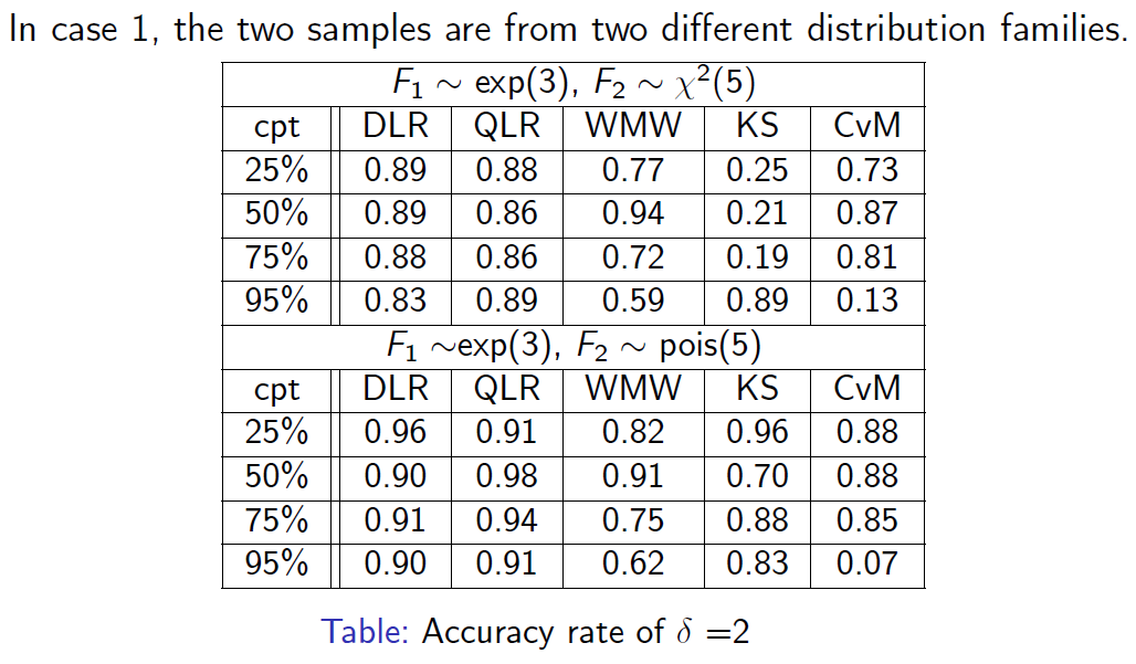
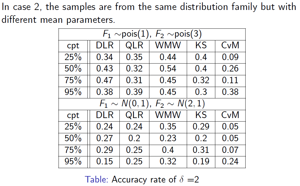
시뮬레이션 결과, DLR이 다양한 분포와 여러 위치에 대해 전반적으로 우수한 성능을 보임을 확인할 수 있었습니다.
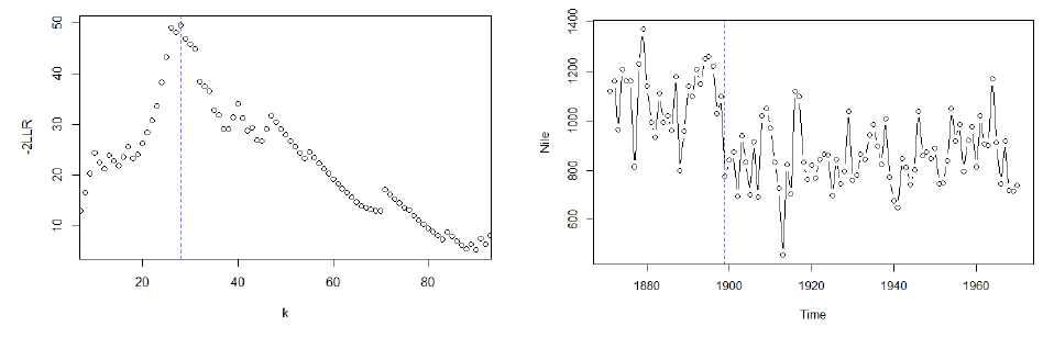
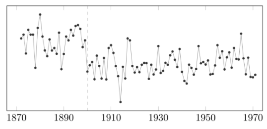
변경점 분석에 널리 연구된 Nile 데이터를 대상으로 DLR을 적용한 결과입니다. 왼쪽 plot은 DLR의 -2LLR입니다. max값인 28이 $\tau$로 추정되었습니다. 이는 오른쪽의 plot을 보았을 때, 1899년까지와 그 이후의 유량은 눈으로도 차이가 보이며 변경점을 잘 탐지했음을 확인할 수 있습니다. (논문에 따르면 1898년에 기후 변화와 Nile강 주변 Aswan 댐의 개입이 1898년에 발생했음을 언급합니다.) 추가적으로 Quantile이 1개일 때와 2개일 때의 Empirical CDF와 p-value에 대한 비교는 아래 첨부자료 Appendix.B에서 확인할 수 있습니다.
4. Outro
본 연구는 제조업 공정, 전력 수요, 금융 등에서 이상이 발생하여 이후 분포가 달라진 경우 그 변경점을 탐지하고 통계적 관점에서 이를 해석할 수 있는 가능성을 제시합니다. 예를 들어, 제조 공정에서 발생하는 다양한 변수(예: 온도, 압력, 속도 등)의 변화가 제품 품질에 영향을 줄 수 있습니다. 제안된 방법은 스트리밍 데이터에 대해 즉각적으로 대응하는 것은 아니지만, 데이터가 쌓이면서 생산 라인에서 발생한 중요한 변경 지점을 정확히 식별하고 품질 문제의 원인을 찾아낼 수 있습니다. 공정의 안정성과 품질에 영향을 미친 요인을 파악하는 분석을 통해 공정 개선의 방향을 설정하고, 공정 조건의 변경이나 장비의 유지 보수 시점을 결정하는 데 도움을 줄 수 있습니다.
References
- Chen, J. and Gupta, A. K. (2011). Parametric statistical change point analysis: with applicationsto genetics, medicine, and finance. Springer Science Business Media.
- Jing, B.-Y. (1995). Two-sample empirical likelihood method.Statistics & probability letters, 24(4):315-319.
- Owen, A. B. (1988). Empirical likelihood ratio confidence intervals for a single functional.Biometrika, 75(2):237-249.
- Owen, A. B. (2001). Empirical likelihood. Chapman and Hall/CRC. * Ross, G. J. and Adams, N. M. (2012). Two nonparametric control charts for detecting arbitrary distribution changes. Journal of Quality Technology, 44(2):102-116.
- Zhang, J. (2002). Powerful goodness-of-fit tests based on the likelihood ratio.Journal of the Royal Statistical Society: Series B (Statistical Methodology), 64(2):281-294.
- Zhang, J. (2006). Powerful two-sample tests based on the likelihood ratio.Technometrics, 48(1):95-103.
- Zhou, Y., Fu, L., and Zhang, B. (2017). Two non parametric methods for change-point detection in distribution.Communications in Statistics-Theory and Methods, 46(6):2801-2815.
-
Zou, C., Liu, Y., Qin, P., and Wang, Z. (2007). Empirical likelihood ratio test for the change-point problem.Statistics probability letters, 77(4):374-382.
- 이미지 출처
- 1: https://en.wikipedia.org/wiki/Control_chart
- 2: https://community.jmp.com/t5/JMPer-Cable/New-features-in-CUSUM-control-charts-for-JMP-16/ba-p/382920
2019년 10월 22일 연세대학교 대우관 본관에서 연구 논문의 예비심사가 진행되었으며 당시 발표에 사용한 자료를 첨부합니다.